

Reinforcement learning basics
I set out to write a post diving into the depths of the Explore-Exploit Dilemma and Multi-armed Bandit problem in reinforcement learning. I created a basic bandit machine model in Python to play with and better understand the basics. This post serves as a personal reminder of the journey, and a guide for others looking to navigate the maze of reinforcement learning methods.
CONTENTS:
1. The multi-armed bandit problem
2. Explore-exploit dilemma
3. Algorithms to solve the dilemma
3.1 Epsilon greedy
3.2 Optimistic initial values
3.3 Upper confidence bound (UCB1)
3.4. Thompson Sampling (Bayesian Bandit)
Conclusion
References and links
1. The multi-armed bandit problem
A multi-armed bandit is a problem in reinforcement learning where an agent must choose between multiple options (the "arms" of the "bandit"), with each option having a potentially different reward. The agent must balance exploration (trying different options to learn more about their rewards) and exploitation (choosing the option with the highest known reward) in order to maximize its overall reward.
A multi-armed bandit can be thought of as a simplified version of an Markov decision process (MDP), where the agent's actions only affect the immediate rewards it receives and not the future states of the environment. The agent's goal is still to find the optimal policy that maximizes its expected cumulative reward, but the problem is simpler because the agent does not have to take into account how its actions will impact future states of the environment.
A multi-armed bandit in Python
I developed a basic bandit machine in Python to experiment with and break down the fundamentals of RL methods.
class bandit_machine:
    """
    class to create a bandit machine object
    """
    def __init__(self, name: str, probability: float):
        """
        Contructor to initialize a bandit machine
        :var name: name of the machine
        :var probability: probabilty to gain a reward
        """
        self.name = name    # Name of the machine
        self.p = probability    # Probability to gain a reward
        self.p_estimated = 0    # Estimated probability for each iteration
        self.n_samples = 1  # Number of times we pull the arm
        self.p_estimated_cache = [0]    # Not need it. Only to plot the sample mean later on

    def pull(self) -> int:
        """
        Method to simulate a result after pulling the arm from the machine
        :return: 1 if you got a reward, 0 if you didn't
        """
        return int(rnd.random() < self.p)

    def update(self, x: int):
        """
        Method to update the estimated probability and number of samples parameters
        """
        self.n_samples += 1
        self.p_estimated = ((self.n_samples - 1) * self.p_estimated + x) / self.n_samples
        self.p_estimated_cache.append(self.p_estimated)
2. Explore-exploit dilemma
The explore-exploit dilemma is a fundamental problem in reinforcement learning that refers to the trade-off between gathering information about the different options available to an agent and maximizing the immediate reward by exploiting the current best option. In simple terms, it is the decision of choosing between trying something new or sticking to what you know. This dilemma arises because there is a trade-off between exploration and exploitation: the more the agent explores, the less it exploits, and the less it explores, the more it exploits. Finding the right balance between exploration and exploitation is crucial to achieve the best overall performance in reinforcement learning.

Explore-exploit dilemma
The Explore-exploit dilemma is the trade-off between gathering information and exploiting the best option in decision-making and reinforcement learning.
3. Algorithms to solve the dilemma
Understanding the sample mean is important in basic reinforcement learning methods like epsilon-greedy because it allows us to estimate the true mean reward of an action.
A naive sample mean approach in reinforcement learning can be problematic because as the algorithm runs for an extended period, the number of rewards stored can become very large and take up a significant amount of memory. This can lead to the algorithm slowing down or even crashing if the memory becomes full.
Starting from the sample mean equation we can calculate the sample mean using constant time and space.
\bar{X}_N = \frac{1}{N} \sum_{i=1}^{N} X_iAn alternative approach to calculating the sample mean in reinforcement learning is to use a constant space and time algorithm by updating the previous sample mean with each new reward received, rather than storing all past rewards.
\bar{X}_N = \frac{1}{N} \sum_{i=1}^{N} X_i ; \quad
\bar{X}_{N-1} = \frac{1}{N-1} \sum_{i=1}^{N-1} X_i;
To do so we can start by spliting the sample mean equation Xi -> X(i-1) + XN
\bar{X}_N = \frac{1}{N} (\sum_{i=1}^{N-1} X_i + X_N)Now we can leave the sum in one side of the equation
\bar{X}_{N-1} = \frac{1}{N-1} \sum_{i=1}^{N-1} X_i \Leftrightarrow \sum_{i=1}^{N-1} X_i = \bar{X}_{N-1} (N-1)And finally we solve the equation:
\boxed{\bar{X}_{N} = \frac{\bar{X}_{N-1} (N-1) + X_N}{N}}This is known as the online sample mean method. It avoids the problem of running out of space to store rewards and it's less computationally expensive than storing all past rewards.
3.1 Epsilon greedy
The Epsilon-Greedy method is a simple algorithm that addresses the explore-exploit dilemma in reinforcement learning. It works by choosing a random action with a small probability (epsilon) and the greedy action with a high probability (1-epsilon). The greedy action is the action that has the highest expected reward, while the random action is chosen uniformly at random.
The idea behind this method is that with a high probability (1-epsilon), the agent will exploit the current best action, maximizing the immediate reward, but with a small probability (epsilon), the agent will explore other actions, gathering information about their rewards to improve future decisions. By balancing exploration and exploitation in this way, the agent can achieve a good trade-off between maximizing immediate rewards and gathering information about the environment, allowing it to make better decisions over time.
This algorithm is simple to implement, computationally efficient and flexible, it can be adjusted by changing the value of epsilon to find the best balance between exploration and exploitation for a particular problem.
Epsilon-Greedy method is an algorithm that balances exploration and exploitation by choosing a random action with a small probability and the greedy action with a high probability, to gather information about the environment and make better decisions over time.
Epsilon greedy in action
The following code creates a simulation of 3 bandit machines with different probabilities of winning. The simulation runs 1000 times, with a 10% chance of randomly selecting a machine and 90% chance of selecting the machine with the highest estimated probability of winning. The code keeps track of the rewards and updates the estimated probability of winning for each machine. The final output shows the estimated probability and a graph of the changes in the estimated probability over time for each machine.
# Create the bandit machines
probabilities = [0.35, 0.5, 0.75]
machines = [bandit_machine(f'machine_{i+1}', p) for i, p in enumerate(probabilities)]

# Initial parameters
n_experiments = 1000
epsilon = 0.1

# Experiment
for i in range(n_experiments):
    # Select the machine to run
    if rnd.random() < epsilon: # Explore action
        selected_machine = machines[rnd.randint(0,2)]
    else:
        best_estimation = max([m.p_estimated for m in machines])
        selected_machine = [m for m in machines if m.p_estimated == best_estimation][0]

    # Pull the machine
    reward = selected_machine.pull()
    selected_machine.update(reward)
After running the experiment we can get the next outputs for each machine.
Machine 1:
machine_1 (39 pulls):
The bandit has a estimated probability of 0.29/0.35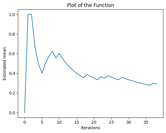
Bandit machine 1
Machine 2:
machine_2 (40 pulls):
The bandit has a estimated probability of 0.46/0.5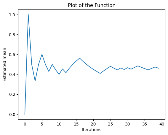
Bandit machine 2
Machine 3:
machine_3 (924 pulls):
The bandit has a estimated probability of 0.77/0.75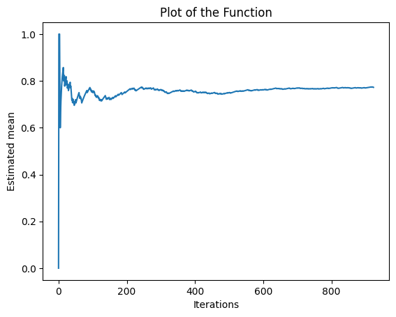
Bandit machine 3
The previous plots shows the estimated mean of the probability of gaining a reward for each bandit machine as the number of iterations increases.
The y-axis represents the estimated probability and the x-axis represents the number of iterations. As the number of iterations increases, the estimated mean converges to the actual probability of the machine to gain a reward.
As the epsilon greedy method balances exploration and exploitation, in the early iterations, the algorithm explores the different machines, leading to more iterations for the machine with higher probability of gaining rewards as it's considered the best option. As the algorithm progresses, it exploits this knowledge, leading to higher iterations for the best machine.
3.2 Optimistic initial values
Optimistic Initial Values is a method that addresses the exploration-exploitation trade-off in Multi-Armed Bandit problems by setting the initial estimates of the rewards for each action to be higher than their actual expected value. The idea behind this method is that by starting with high estimates, the agent will be more likely to explore actions that it initially thinks have high rewards, leading to a faster convergence to the true optimal action.
The main difference between Optimistic Initial Values and Epsilon-Greedy method is how they balance exploration and exploitation. Epsilon-Greedy method does it by choosing a random action with a small probability and the greedy action with a high probability. On the other hand, Optimistic Initial Values does it by setting the initial estimates of the rewards for each action to be higher than their actual expected value, leading to a higher probability of exploration.
In summary, the Epsilon-Greedy method is based on balancing exploration and exploitation by randomizing the action choice, while the Optimistic Initial Values method is based on guiding the exploration by starting with optimistic estimates of the rewards. Both methods can be used to find the optimal action in Multi-Armed Bandit problems, but they use different strategies to balance the exploration and exploitation trade-off.
Optimistic Initial Values is a method that addresses the exploration-exploitation trade-off in Multi-Armed Bandit problems by setting initial estimates of rewards higher than their actual value, leading to more exploration and faster convergence to the optimal action.
Optimistic initial values in action
We can modify the previous machine by setting the initial estimated probability in 2 to see the Optimistic Initial Values approach.
For this example we set the parameter p_estimated to 2
self.p_estimated = 2.and we run 200 experiments obtaining a comparison with the Epsilon Greedy plot.

Epsilon greedy VS Optimistic initial values
As a reminder, Epsilon-greedy is a more general method while Optimistic Initial Values is a specific strategy. In some cases, Optimistic Initial Values may perform better, but in other cases, epsilon-greedy may be more suitable. It's important to test and evaluate both methods in the specific context.
3.3 Upper confidence bound (UCB1)
Upper Confidence Bound (UCB1) is a method that addresses the exploration-exploitation trade-off in Multi-Armed Bandit problems by choosing actions based on the estimated potential reward and the degree of uncertainty associated with that estimate. The idea behind this method is that at each time step, the agent should choose the action that has the highest upper confidence bound, which is calculated as the average reward plus a term that accounts for the degree of uncertainty.
The main difference between UCB1 and Optimistic Initial Values is that while Optimistic Initial Values sets the initial estimates of the rewards for each action to be higher than their actual expected value, leading to more exploration, UCB1 uses the Hoeffding inequality to calculate the upper confidence bound for each action, it balances exploration and exploitation by choosing actions based on the estimated potential reward and the degree of uncertainty associated with that estimate.
In summary, Optimistic Initial Values uses high initial estimates to guide exploration, while UCB1 uses estimates of potential rewards and uncertainty to guide the exploration-exploitation trade-off.
Upper Confidence Bound (UCB1) is a method that addresses the exploration-exploitation trade-off in Multi-Armed Bandit problems by choosing actions based on the estimated potential reward and the degree of uncertainty associated with that estimate, leading to an optimal balance between exploration and exploitation.
UCB1 theory
The upper confidence bound is calculated as the average reward of an arm plus a term that accounts for the uncertainty of the estimate, which is typically the square root of the inverse of the number of times the arm has been pulled. This allows the algorithm to balance the need for exploration to improve estimates of the true rewards with the need for exploitation to maximize rewards.
We can use this made-up function to illustrate the idea:
p(sampleMean - trueMean \geq error) \le f(error)The function represents the probability that the difference between the sample mean (estimated mean) and the true mean (actual mean) of the rewards is greater than a certain error, with f(t) being a decreasing function that depends on the desired level of confidence. The UCB algorithm uses this function to determine the upper bound on the error, which is used to select the arm to play. In short, it represents the probability that the arm selected by UCB is not the best one.
p(\bar{X}_n - E(X) \geq t) \le f(t)If the function (f(t)) is a decreasing function, it means that as the error value gets smaller, the probability of a big error becomes smaller, while the probability of a small error becomes bigger. This is because as the number of samples increases, the sample mean becomes a better estimate of the true mean, and the degree of uncertainty in that estimate decreases, making it less likely that a large error will occur.
The decreasing function:
-
Markov Inequality: the function decreases proportional to 1/t
p(\bar{X}_n - E(X) \geq t) \le \frac{1}{t} -
Chebyshev Inequality: the function decreases faster proportional to 1/t^2.
p(\bar{X}_n - E(X) \geq t) \le \frac{1}{t^2} -
Hoeffding's inequality: the function decreases faster than any polynomio proportional to e^(-2nt^2)
p(\bar{X}_n - E(X) \geq t) \le e^{-2nt^2}We are going to use the Hoeffding's inequality in our model.
Upper Confidence Bound (UCB1) in action
Before diving into the code, I want to provide a high-level overview of the algorithm by presenting a pseudocode, which will help to better understand how the equations are implemented in the actual code.
Loop:
\boxed{j = max( \bar{X}_{nj} + \sqrt{ 2 \frac{\log{N}}{n_j} })} \\
 \bar{X}_{nj}: \textrm{mean from j machine} \\
N: \textrm{total plays made} \\
n_j: \textrm{plays made on j machine}
The code only needs to update the way the bandit machine is selected by adding the weight from Hoeffding's inequality, without modifying the rest of the code.
By creating the function apply_weight, it applies the weight derived from the Hoeffding's inequality to estimate the upper confidence bound of a sample mean x_mean, based on the number of plays n_plays and the number of samples n_samples.
def apply_weight(x_mean, n_plays, n_samples):
    return x_mean + (2*log(n_plays)/n_samples)**0.5
The code selects the best machine in each iteration of the loop by applying the weights and updating the way the bandit machine is chosen.
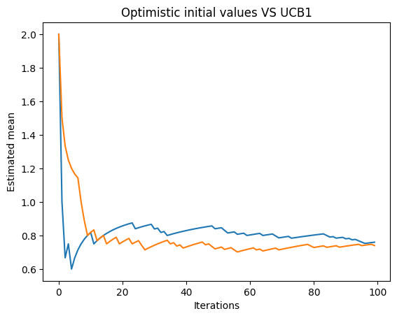
Optimistic initial values (blue), UCB1 (orange)
In the next plot, we can see two lines. The blue line represents the estimated mean obtained using the optimistic initial values method, and the orange line represents the estimated mean obtained using the UCB1 method. The plot helps us visualize the convergence of the estimated means towards the actual probability of gaining a reward for each bandit machine.
3.4 Thompson Sampling (Bayesian Bandit)
Thompson Sampling is a method for solving Multi-Armed Bandit problems that addresses the exploration-exploitation trade-off by sampling actions from their posterior distributions. It works by maintaining a prior distribution for the expected reward of each action, and then using Bayesian update rules to update these distributions as new data is obtained. At each time step, the agent samples from these distributions, and chooses the action with the highest sample as the next action.
- Small dataset -> Large confidence interval, and vice versa.
- Skinny confidence interval -> more exploting and less exploring.
The main difference between Thompson Sampling and UCB1 is that UCB1 uses the estimates of expected rewards and their uncertainty to guide the exploration-exploitation trade-off, while Thompson Sampling uses the Bayesian update rule to maintain posterior distributions of the expected rewards, and samples from these distributions to guide the exploration-exploitation trade-off.
Thompson Sampling is a method for solving Multi-Armed Bandit problems that addresses the exploration-exploitation trade-off by sampling actions from their posterior distributions, using Bayesian update rules to choose the action with the highest sample as the next action.
Thompson Sampling Theory
To understand Thompson Sampling, it is important to have a basic understanding of Bayes rule, which is a way to update our beliefs about the probability of an event based on new data.
The Bayes rule formula is:
posterior = \frac{prior X likelihood}{evidence} \\
---\\
\boxed{P(\theta | X) = \frac{P(\theta | X) P(\theta)}{P(X)}}
The prior represents our initial belief about the probability of an event, the likelihood is the probability of observing the data given the event, and the evidence is the total probability of observing the data.
The approach is based on Bayesian probability to choose the best bandit. Alpha and beta shape the beta distribution as the posterior distribution of each bandit's reward. The bandit with the highest expected reward is selected by sampling from the updated posterior distribution based on observed rewards.
Thompson Sampling in action
Thompson Sampling with Gaussian reward theory
Thompson Sampling with Gaussian reward theory is a variant of the Thompson Sampling algorithm that assumes rewards follow a Gaussian distribution, it uses Bayesian update rules and samples from distributions to choose actions, it is more efficient and allows for calculation of rewards uncertainty.
Thompson Sampling with Gaussian reward in action
Comming soon!
Conclusion
In conclusion, the previous conversation covered several basic reinforcement learning methods including Epsilon Greedy, Optimistic Initial Values, Upper Confidence Bound (UCB1), and Thompson Sampling (Bayesian Bandit).
Epsilon-greedy is a simple method that balances exploration and exploitation. It is useful when the rewards are relatively stable and the goal is to find the best action quickly.
Optimistic Initial Values is a method that starts with high estimates of the rewards of each action, it is useful when the rewards are highly variable and the goal is to quickly discard bad actions.
Upper Confidence Bound (UCB1) is a method that balances exploration and exploitation by considering not only the average reward but also the uncertainty of the estimates. It is useful when you have a prior belief about the expected rewards of each action and the goal is to find the best action while minimizing the regret.
Thompson Sampling (Bayesian Bandit) is a method that considers the uncertainty of the estimates by modeling the rewards as a probability distribution. It is useful when you have a prior belief about the distribution of rewards for each action and the goal is to find the best action while minimizing the regret.